GAN Deep Dive - Part 1
There have been a lot of recent HTC posts on the deep learning GAN architecture. Let's take a deep dive into how to code up different GAN architectures using the fastai api.
We're going to have several different posts that run through a number of different approaches to building GAN models. Keep in mind that the GAN sub field of deep learning is changing rapidly as more and more research is done. So we're going to be working through some of the historical developments in this series of posts.
Part 1 starts with Lecture 12 of the 2018 fastai course. The lecture starts off with taking a look at the DarkNet architecture used in YOLOv3. This is very interesting stuff, so feel free to check it out. But it doesn't really have anything to do with GANs directly.
The lecture then focuses on Generative Adversarial Networks (GAN) from 48.38 onwards. This later part of the lecture is our focus for this particular GAN Deep Dive post.
It starts by taking a look at the DCGAN architecture discussed in this paper.
It then moves on to discussing the Wasserstein GAN. The Wasserstein GAN paper (and this followup paper) is really all about making GANs easier to train and more stable during training (avoiding mode collapse). You can think of mode collapse as a kind of overtraining, where the system memorizes a few specific correct output choices and then always generates them rather then the infinite variety of unique different outputs you really want the GAN system to generate.
Jeremy shows you how to code up both the DCGAN and the Wasserstein GAN using fastai api (v1, not v2).
He then shows off a fun graphical animation of how Convolution works as a lead in to talking about DeConvolution. Many early GAN papers had a visual checkerboard artifacts in their generated image outputs, he discusses why this occurred and how to get rid of it.
There's a great Distil article on Deconvolution and Checkerboard Artifacts he points out that you can read here.
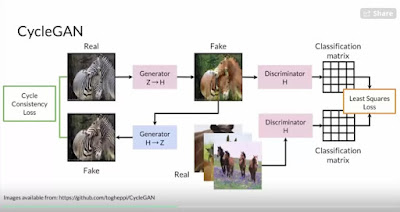
Jeremy then moves onto covering the CycleGAN architecture. To get you up to speed on CycleGAN (or jog your memory if it seems familiar), we present a CycleGAN 2 Minute Paper Presentation below.
CycleGAN is pretty mind boggling when you first hear about it. The classic example of what you could do with CycleGAN is to train a system to automatically make horses look like they have zebra stripes.
Other examples might include taking a Monet painting and generating what the real world scene he painted might have looked like. Or automatically changing the sky in a photo from daytime to nighttime (or making a photo of a dry scene look like it is a wet rainy scene).
So the CycleGAN introduces the concept of using a GAN to visually edit an image (modify that image in some controllable way). You can read the original CycleGAN paper here.
Jeremy uses the code library from the original CycleGan paper above to implement his CycleGAN model. Probably because the paper only came out a few days before the lecture. He implements all of it in fastai api in a 2019 lecture in the upcoming Part 2 post of this series.
Here is a link to a very good blog post on Understanding and Implementing CycleGAN in TensorFlow.
The power of the CycleGAN architecture is the ability to learn image transformations without needing to have explicit one-to-one mapping data examples to train the model.
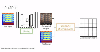
Note that this is different from other transformational models like Pix2Pix that require paired source-output data.
Some Observations
1: A big part of the history of GAN development involves working through different loss functions to use in the deep learning associated with the model to get better results.
Remember, any deep learning system is only going to optimize what you tell it to. And the loss function you are using in the deep learning model is what you are telling it to do. Using a crappy loss function for your particular problem equals crappy output from your badly trained model.
2: The Wasserstein loss function is really an approximation of something called Earth Movers distance. A great intuitive way to think about Earth Movers Distance is that it measures the amount of work you have to do to physically move one probability distribution to fit another probability distribution.
Jeremy does not discuss this in the lecture, and i really think it's the easiest way to understand what is going on in the Wasserstein loss function. BCE loss was originally used in GAN research, and Wasserstein loss was developed to try and overcome the limitations associated with BCE loss when training GAN models.
The 2nd Wasserstein GAN paper i mentioned above introduced a second trick, which is to clip the ends of the probability distribution. Clipping the weights of the network in practice. An alternative was to do is is to penalize large gradient values. Both of these are trying to ensure 1-Lipschitz continuity (1L continuity). You can think of penalizing large gradients as a soft way of doing weight clipping.
3: A Min-Max optimization objective is important in the CycleGAN work. What Min-Max means is that the system is trying to minimize one objective while it maximizes the other objective.
Where have you heard this principal before (competing objectives fighting it out)?
4: The fastai api and fastai courses are moving targets in some sense. Which is no different then the rest of the deep learning field. Things are changing at a very rapid pace.
Are there specific features associated with recent GAN research that still need to be implemented and incorporated into the fastai 2 api that addresses GANs?
5: We're using GAN systems that work with images in this post, but you certainly aren't restricted to only using GANs on imaging problems. The underlying principals being discussed in all of the HTC GAN posts can be applied to many different problem domains.
How can you use a GAN in a problem domain you are specifically interested in?


Comments
Post a Comment